How Do I Do Land-Use Change Analysis? GIS Methods for Site Planning
Land-use change analysis in GIS is done by collecting satellite images of the same area from different dates, classifying the land into categories such as built-up areas, vegetation, farmland, bare land, and water bodies, and comparing the results to measure what has changed over time. For site planning, this helps you identify development trends, environmental risks, and unsuitable land before investing in a property.
A client once sent me coordinates for a plot he’d agreed to buy in a fast-growing part of Akwa Ibom. On Google Maps, it looked fine: flat, cleared, and close to a new road. What he didn’t know, because nobody had checked, was that the same spot had been a seasonal wetland three years earlier, and the “clearing” was recent sand-filling, not naturally dry ground. I downloaded satellite imagery from three different years, classified the land-cover types, and compared the results. The analysis revealed evidence of previous water coverage exactly where he planned to build. He avoided losing his deposit and renegotiated for a different plot on the same layout.
This is what land-use change analysis does in practice. It answers a critical question: how has this land changed, and what do those changes mean for your proposed development? Whether you are a student working on a research project, a GIS professional providing mapping services, or a property buyer assessing a building site, the process follows a clear workflow. You acquire suitable satellite images, prepare them for analysis, classify land cover, compare different periods, calculate the changes, and produce maps showing the results. Tools such as QGIS, Google Earth Engine, and remote-sensing datasets from Landsat or Sentinel-2 can support this process. In this guide, you will learn the GIS methods, change-detection techniques, calculations, statistics, and map-production steps needed to perform land-use change analysis for informed site planning.
What Land-Use Change Analysis Actually Is (In Plain Terms)
Land-use change analysis is the process of comparing how a specific piece of land was classified and used at two or more points in time, to measure what changed, how much changed, and where exactly the change happened. It sits inside the broader field of remote sensing and GIS, but you don’t need to be a GIS specialist to understand the logic: you’re looking at the same location in Year 1, Year 2, and Year 3 (or further back), classifying what’s on the ground each time vegetation, built-up area, bare soil, water, farmland and then measuring the difference between those classifications.
This matters for three very different audiences at once, and that’s exactly why it deserves a proper guide rather than a quick blog paragraph:
Researchers and students use it to study urban sprawl, deforestation, wetland loss, or agricultural conversion over a defined period, usually for a thesis, a consultancy report, or a government planning document.
GIS and planning professionals increasingly offer it as a standalone paid service land-use change reports for due diligence, environmental impact screening, or litigation support.
Ordinary people planning to build which is the audience this website exists for can use a simplified version of this same analysis to check whether a plot they’re about to buy has a land-use history that should worry them, long before a surveyor or a lawyer ever gets involved.
Now that the destination is clear, let’s walk through how you actually get there starting with the part everyone gets wrong first: picking your time points.
Step 1: Choosing Your Time Points (Year 1 → Year 2 → Year 3)
Every land-use change study is built around at least two time points, but three gives you something two can’t: a trend, not just a snapshot. Two dates tell you something changed. Three dates tell you whether that change is accelerating, slowing down, or reversing which is the difference between a study that describes the past and one that can actually inform a decision about the future.
A practical way to choose your three years:
Year 1 (Baseline) as far back as reliable imagery allows for your area. For most of the world, that’s realistically 10-20 years back using freely available satellite data.
Year 2 (Midpoint) roughly halfway between Year 1 and today, used to catch a change that happened early and then stabilized, versus one that’s still actively progressing.
Year 3 (Current/Most Recent) the most recent cloud-free imagery available for your site, ideally within the last 12-18 months.
For a small-plot buyer, a workable set might be 2015, 2020, and 2024. For an academic study, your time points are usually fixed by data availability or by the specific event you’re studying (before/after a government project, a flood, a new road).
With your years chosen, the next question is where that imagery actually comes from and this is where most guides either get too technical too fast, or stay so vague they’re useless.
Step 2: Getting Your Data (Free and Paid Sources)
You don’t need an expensive subscription to do a credible land-use change analysis. Here’s what’s actually available, organized by what it’s good for:
Landsat (USGS Earth Explorer) free, going back to the 1970s-80s depending on location, 30-metre resolution. Good for broad land-use categories (built-up vs. vegetation vs. water) over long time spans.
Sentinel-2 (Copernicus/ESA) free, available from 2015 onward, 10-metre resolution. Better detail than Landsat for a specific plot or neighbourhood-scale study.
Google Earth historical imagery free, variable resolution and inconsistent dates, but excellent for a quick visual gut-check before committing to a full technical analysis.
National mapping agency data this is where it gets interesting depending on where you are, which matters a great deal for this site’s audience, since readers come from Nigeria, the US, UK, Germany, UAE, Iceland, Luxembourg, Switzerland, Qatar, Canada, Australia, and Singapore, among other places.
Here’s a quick reference for where to pull authoritative land-use/land-cover data by country, useful whether you’re analyzing land there directly or just want to understand how your own country’s planning authority classifies land:
| Country/Region | Key Data Source |
|---|---|
| Nigeria | NASRDA/NigeriaSat imagery, State Geographic Information Systems (GIS) agencies |
| United States | USGS National Land Cover Database (NLCD) |
| United Kingdom | Ordnance Survey, UKCEH Land Cover Maps |
| Germany & EU | CORINE Land Cover (Copernicus Land Monitoring Service) |
| Switzerland | Swisstopo (Federal Office of Topography) |
| Canada | Canada Land Cover (Natural Resources Canada) |
| Australia | Geoscience Australia, Digital Earth Australia |
| Singapore | Singapore Land Authority (SLA), URA Master Plan portal |
| UAE & Qatar | Municipal GIS portals (Dubai Municipality GIS, Qatar GIS Portal) |
| Iceland, Luxembourg | National mapping agencies (Landmælingar Íslands, Administration du Cadastre et de la Topographie) |
Wherever you are, the underlying method below applies the same way only the data source name changes. That consistency is actually the point: land-use change analysis is a universal GIS technique, not a Nigeria-specific trick, which is exactly why it transfers so cleanly whether you’re screening a plot in Uyo or double-checking a flood-prone parcel in Houston.
Once your imagery is in hand for all three years, the real work begins: turning raw images into classified land-use maps you can actually compare.
Step 3: Classifying Each Year’s Land Use
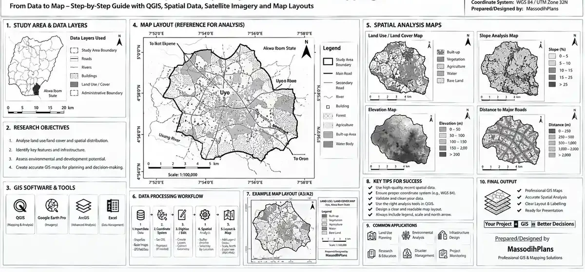
Classification means assigning every part of the image to a land-use/land-cover category. For a small-plot study, you don’t need the full academic classification system a simplified version works well:
Simplified Classification Scheme (Anderson Level I-style):
- Built-up/Developed land
- Vegetation (forest, farmland, grassland)
- Bare soil/Cleared land
- Water bodies/Wetland
- Other (roads, bare rock, etc.)
For each of your three years, you classify the image using one of two approaches:
Visual/manual classification looking at the imagery and manually marking boundaries between categories. Slower, but accessible with free tools like QGIS and no coding knowledge.
Supervised classification using software (QGIS’s Semi-Automatic Classification Plugin, or similar tools) to automatically classify pixels based on sample training areas you define for each category. Faster and more consistent for larger study areas.
For a single small plot and its immediate surroundings, manual classification is genuinely sufficient and is what I use for most client due-diligence reports you don’t need machine-learning-grade rigor to answer “was this a wetland five years ago.”
Three classified maps on their own are informative, but they don’t yet tell you the one number everyone actually wants: how much changed, and by how much. That’s where change detection comes in and this is where the formulas earn their place in this guide.
Step 4: Change Detection — The Formulas That Actually Matter
This is the section most land-use articles skip entirely, or handle so abstractly that a reader can’t actually use it. Here are the calculations that turn your classified maps into real numbers.
Formula 1: Area Change
Area Change (ΔA) = Area in Year 2 − Area in Year 1
This gives you the raw change in hectares or square metres for any land-use category between two time points.
Formula 2: Percentage Change
Percentage Change (%Δ) = [(Area Year 2 − Area Year 1) ÷ Area Year 1] × 100
Example: if built-up area around your study plot was 12 hectares in 2015 and is 19 hectares in 2024:
%Δ = [(19 − 12) ÷ 12] × 100 = 58.3% increase in built-up area over 9 years
Formula 3: Annual Rate of Change (Compound)
This is more useful than a flat percentage because it accounts for time span, letting you compare a 5-year study to a 15-year study fairly.
r = [(A2 ÷ A1)^(1/t) − 1] × 100
Where A1 = area at Year 1, A2 = area at Year 2, and t = number of years between them.
Using the same example (12 hectares to 19 hectares over 9 years):
r = [(19 ÷ 12)^(1/9) − 1] × 100 ≈ 5.2% per year
A 5.2% annual rate of built-up land expansion around a plot is a meaningful early-warning signal it tells you the area is urbanizing fast, which has direct implications for future drainage load, traffic, and infrastructure strain on exactly the kind of small plot this website is built to help people plan on.
Formula 4: Land Consumption/Absorption Rate (for urban sprawl studies)
If you’re studying how efficiently new urban land is being used relative to population growth:
Land Absorption Coefficient (LAC) = (Urban Area Year 2 − Urban Area Year 1) ÷ Population Increase
A rising LAC over time signals urban sprawl (low-density expansion eating more land per new resident) a figure used heavily in academic urban growth studies and genuinely useful for anyone assessing whether an area’s growth pattern is sustainable or just spreading thin.
Formula 5: Change Detection via Image Differencing (for remote sensing students)
For those doing this with actual raster data rather than manual classification:
Difference Image = Band Value (Year 2) − Band Value (Year 1)
Pixels with values close to zero indicate no change; strongly positive or negative values indicate significant change in that location this is the basis of most automated change detection algorithms in GIS software.
Numbers are only trustworthy if your classification was accurate in the first place, which brings us naturally to the step almost every amateur land-use study skips entirely: checking your own work.
Step 5: Accuracy Assessment — Proving Your Analysis Is Actually Reliable
A land-use change map that hasn’t been accuracy-checked is an opinion, not a finding. This is true whether you’re submitting a university thesis or handing a client a due-diligence report they’re about to make a financial decision on.
Overall Accuracy
Overall Accuracy (OA) = (Number of Correctly Classified Points ÷ Total Reference Points) × 100
You check this by comparing your classified map against known reference points ground-truth data, high-resolution imagery, or local knowledge of what’s actually at specific locations.
Kappa Coefficient
This is the gold-standard accuracy statistic in land-use studies because it accounts for the accuracy that could happen purely by chance:
Kappa (κ) = (Po − Pe) ÷ (1 − Pe)
Where Po = observed agreement (your overall accuracy as a proportion) and Pe = expected agreement by chance.
As a rule of thumb used across GIS practice: a Kappa value above 0.80 is considered strong agreement, 0.60-0.80 is substantial, and below 0.40 means your classification isn’t reliable enough to base real decisions on. If you’re delivering this as a paid service, quoting your Kappa value is what separates a credible report from a guess with a nice-looking map attached.
With your changes measured and your accuracy proven, the last step is presenting it in a form other people a client, a thesis supervisor, a planning authority can actually use. That means a transition matrix and a map.
Step 6: The Transition Matrix (What Changed Into What)
A transition matrix is a table showing exactly which land-use category converted into which other category between two time points. This is more useful than a simple percentage change, because it tells you the story behind the number.
Example transition matrix (Year 1 to Year 3, in hectares):
| From ↓ / To → | Built-up | Vegetation | Bare Soil | Water/Wetland |
|---|---|---|---|---|
| Built-up | 10.2 | 0.1 | 0.3 | 0.0 |
| Vegetation | 4.8 | 15.6 | 1.2 | 0.2 |
| Bare Soil | 2.1 | 0.4 | 3.0 | 0.1 |
| Water/Wetland | 1.9 | 0.3 | 0.6 | 2.8 |
Reading this table: 4.8 hectares of what was vegetation in Year 1 became built-up by Year 3 that’s urban expansion into green land. More importantly for a plot buyer, 1.9 hectares of what was water/wetland in Year 1 became built-up by Year 3 that’s exactly the pattern my client’s plot showed, and exactly the pattern a transition matrix makes impossible to miss.
Step 7: Producing the Final Maps
The final deliverable whether for a thesis, a paid client report, or your own due diligence is a set of maps that make the change visually obvious at a glance:
Three classified maps, one per year, using a consistent colour scheme across all three so a reader can flip between them and see the pattern
One change map, typically showing “no change” in grey and highlighting specific transitions (e.g., vegetation-to-built-up in red, water-to-built-up in a distinct colour) so the riskiest changes jump out immediately
A summary statistics panel alongside the map area change, percentage change, and annual rate of change for each category, pulled directly from the formulas above
A map without the numbers looks impressive but can’t be rigorously defended. Numbers without the map are hard for a non-technical client to actually act on. Together, they’re what makes a land-use change analysis genuinely decision-grade rather than just interesting.
Why This Matters Specifically If You’re Planning to Build on a Small Plot
Everything above is standard GIS methodology but here’s the part that connects it back to what this website actually exists to help you do: build well on a small plot, without discovering an expensive surprise after construction has started.
A proper land-use change analysis on a plot you’re considering tells you things a single site visit never will:
Was it ever a wetland, floodplain, or drainage path? Sand-filled land doesn’t behave like naturally dry land it settles differently, drains differently, and can resurface flooding problems years after you’ve built, regardless of how solid your foundation design is.
Is the surrounding area urbanizing faster than its infrastructure can handle? A high annual rate of change in built-up land around your plot is an early signal of the exact infrastructure-strain problem covered in our guide on how buildings relate to their streets, neighbourhoods, and cities roads, drainage, and power sized for yesterday’s density, carrying tomorrow’s load.
Is agricultural or vegetated land disappearing fast nearby? This often precedes rapid, sometimes poorly planned residential conversion useful context before committing to a small plot in an area that might look quiet today and be a congested, under-serviced neighbourhood in five years.
For diaspora clients especially, this is a way to verify a plot’s history remotely, without relying solely on an agent’s description or a single recent photo, before wiring money for land you haven’t physically walked on in years.
This is also, quite plainly, a genuine service opportunity if you’re a GIS professional, student, or planner reading this rather than a homeowner land-use change due diligence reports are an underexplored, clearly demonstrable value-add you can offer alongside architectural design and building plan services, and it’s one I now build into due-diligence work for clients before any floor plan is even sketched.
A Simple DIY Workflow If You Want to Try This Yourself
- Download QGIS (free, open-source) and install the Semi-Automatic Classification Plugin
- Pull Landsat or Sentinel-2 imagery for your three chosen years from USGS Earth Explorer or Copernicus Open Access Hub, cropped to your area of interest
- Classify each year’s image into the five simplified categories above
- Run the area and percentage change formulas (Steps 4) on each category
- Build your transition matrix comparing Year 1 to Year 3
- Generate your change map, keeping colours consistent across all outputs
- If this is for a paid report or academic submission, run an accuracy assessment against ground-truth points before presenting your findings as final
If you only have time or budget for one comparison, don’t default to “most recent vs. oldest available.” Run Year 1 vs. Year 2 and Year 2 vs. Year 3 separately as well a plot that looks stable overall can hide a sharp change that happened and then paused, which a single start-to-end comparison will completely miss.
A land-use change analysis tells you what happened to the land it does not replace a soil test, a survey plan verification, or formal planning authority approval checks. Treat it as the first due-diligence layer, not the only one, before you commit funds to any plot.
Frequently Asked Questions
What software do I need to do land-use change analysis?
QGIS (free) handles everything from classification to mapping for most small-scale studies. ArcGIS is the paid alternative used more commonly in academic and government settings, but isn’t necessary for a plot-level analysis.
How many years of data do I actually need?
Two time points are the minimum, but three is strongly recommended because it reveals whether a change is accelerating, stable, or reversing, rather than just confirming that something changed.
What’s a good Kappa coefficient for a reliable study?
Above 0.80 is considered strong agreement in most GIS literature. Below 0.40 means the classification shouldn’t be relied on for real decisions, whether academic or practical.
Can I do this without any GIS software, just by comparing satellite photos visually?
Yes, for a quick gut-check Google Earth’s historical imagery slider is genuinely useful for this. But for anything you’re presenting formally, as a paid report, or using to make a significant financial decision, run the proper classification and accuracy steps above.
Is land-use change analysis relevant outside Nigeria?
Completely. The method and formulas are identical everywhere only the data source changes, whether that’s the NLCD in the US, CORINE in Germany, Swisstopo in Switzerland, or a municipal GIS portal in the UAE or Qatar. If you’re screening land anywhere in the world, this same workflow applies.
How is this different from just checking a survey plan?
A survey plan tells you the legal boundaries and dimensions of a plot today. A land-use change analysis tells you the physical history of that land over time what it actually was before it looked the way it does now. You need both, not one instead of the other.
Conclusion
Land-use change analysis sounds like something reserved for research papers and government planning departments, but at its core it answers a question anyone planning to build should be asking anyway: what was here before, and is that history going to cause me a problem later? Three years of imagery, a handful of straightforward formulas, and one transition matrix can surface a risk that a single site visit, however thorough, simply cannot.
If you’re planning a small plot and want this kind of due-diligence layer built into your project from the start, our Services page covers how we combine planning analysis with architectural design before a single wall goes up. Browse our Plans Library for house designs already suited to small Nigerian plots, or visit Plan School to understand the planning and approval steps that come after your site has been properly vetted. You can also explore more planning and GIS guides on our Homepage.
- How Many Plots Can I Get From This Land? Plot Size & Layout Guide
- Can I Build a Church or Mosque on This Land? Check Nigeria’s Rules
- How Do I Check a Property Before I Build? 7 Checks to Avoid Costly Errors
- How Do I Compare Two Properties? Size, Value & Land Checks in Nigeria?
- How Do I Produce GIS Maps for My Project? A Practical Mapping Guide
- How Do I Overlay GIS Layers? Complete QGIS Analysis Guide
Author
Massodih Okon is a Nigerian built-environment professional with academic and professional experience in urban and regional planning, geography, architectural design, Landscape Design, GIS and land development.
He holds a Master’s degree in Urban and Regional Planning from the University of Uyo and a first degree in Geography and Regional Planning.
Through MassodihPlans, he publishes practical guides on Nigerian house plans, building design, physical planning, site planning, development approval and residential construction. Read the full author profile →